Influence of initial increment size on stress–strain results in *STATIC analysis

[TOSHI]

Hello,

I have a question about the influence of the initial increment size in a *STATIC analysis.

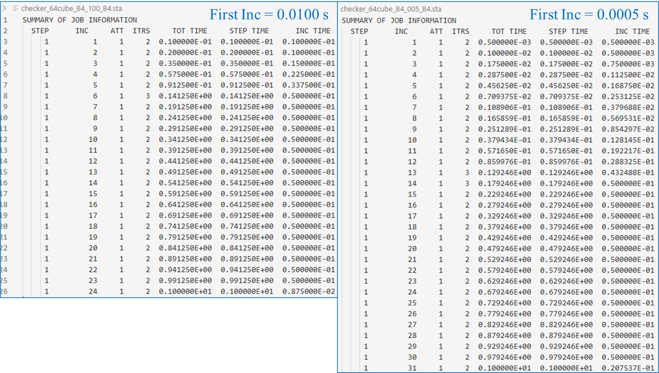
When I change the initial increment, the deformation behavior and the nominal stress–nominal strain curves shift noticeably, as shown in the attached figure. I am running simulations on a cubic RVE, and the material behavior is evaluated based on its constitutive model.

The initial increments I tested are 0.0005, 0.0010, 0.0050, and 0.01 s, and each setting produces a different stress–strain response.

Is it normal for a *STATIC analysis to show such sensitivity to the initial time increment?
Since the step is defined using *STATIC, I expected the results to be relatively independent of the initial increment.

For each case, I change the first parameter of the *Static line (0.0005, 1, 1E-07, 0.05) to set a different initial increment.

Any advice or clarification would be appreciated.

Regards,

Here is the step and boundary condition definition from my .inp file (I could not upload the file, so I paste the relevant part):

** SECTIONS +++++++++++++++++++++++++++++++++++++++++++++
*Solid Section, elset=PART-1-1_FERRITE, material=Ferrite
*Solid Section, elset=PART-1-1_MARTENSITE, material=Martensite
**
** STEP +++++++++++++++++++++++++++++++++++++++++++++++++
*Step, name=Step-1, nlgeom=YES
*Static, Solver=PaStiX
0.0005, 1, 1E-07, 0.05
*Output, frequency=1
** Boundary conditions +++++++++++++++++++++++++++++++++++++
*Boundary, op=New
Internal_Selection-1_X, 1, 1, 0
Internal_Selection-1_X, 5, 5, 0
Internal_Selection-1_X, 6, 6, 0
Internal_Selection-1_Y, 2, 2, 0
Internal_Selection-1_Y, 4, 4, 0
Internal_Selection-1_Y, 6, 6, 0
Internal_Selection-1_Z, 3, 3, 0
Internal_Selection-1_Z, 4, 4, 0
Internal_Selection-1_Z, 5, 5, 0
Internal_Selection-1_ENCASTRE, 1, 1, 0
Internal_Selection-1_ENCASTRE, 2, 2, 0
Internal_Selection-1_ENCASTRE, 3, 3, 0
Internal_Selection-1_ENCASTRE, 4, 4, 0
Internal_Selection-1_ENCASTRE, 5, 5, 0
Internal_Selection-1_ENCASTRE, 6, 6, 0
*Boundary
Internal_Selection-1_Displacement_Rotation-1, 1, 1, 30
...
*End Step

[FEAnalyst]

First of all, you should keep in mind that the initial increment size is just a suggestion for the solver - it may modify it and automatic incrementation will choose increment sizes on its own based on the convergence progress (of course, it will keep them within the specified min-max limit). To have more control over incrementation, you can switch it to Direct - then the specified increment size is kept constant during the analysis. It may lead to non-convergence but if that’s not a problem then give it a try.

Also, it might be good to try with Pardiso - it’s more reliable than PaStiX.

[TOSHI]

Thank you very much for your quick and helpful reply — I really appreciate it.

I understand the behavior of automatic incrementation and the difference between Automatic and Direct modes.

However, my main concern is that the stress–strain response itself changes significantly depending on the initial increment size.

The difference is clearly visible in the first plot I attached — the curves diverge noticeably even though the material model and all analysis settings are identical. This is the part that concerns me the most.

This makes me wonder whether such sensitivity is expected for *STATIC with nonlinear material behavior, or if it indicates an issue such as inaccurate plasticity integration when the increments are too large.

I will try Pardiso as you suggested.

At the moment I am using PaStiX mainly due to runtime constraints, but I will check whether Pardiso gives more consistent results.

If you have any insight into why the mechanical response changes so much with different initial increments, I would be very grateful.

Thanks again for your support.

[FEAnalyst]

Can you share the contents of the Status tab of the job monitor in both cases (to see how the automatic incrementation progresses) ? There are no amplitudes for time variation of loading in this model, right ?

[TOSHI]

Thanks for your reply.
Here are the screenshots from the Status tab showing how the automatic incrementation progresses for both cases.

The left one corresponds to First increment = 0.0100 s,
and the right one corresponds to First increment = 0.0005 s.
As you can see, the incrementation histories differ quite a lot between the two runs.

Regarding your question about amplitudes — there are no amplitudes defined in this model.
The loading is applied directly as a displacement boundary condition, without any time-dependent amplitude.

Since I’m a new user and can’t upload files yet, I will paste the required parts manually if needed.

Thanks again for your assistance.

[ANYS]

Hi,

Are you using Johnson-Cook material model or a custom strain rate material model? They show that behaviour.

Curves are quite similar but “shifted ”. If your model is displacement driven and you don’t have control on the incrementation your cube could be under different strain rates.

Below an example of how curves look like .

[Sound_Spinning]

You should switch to ‘load driven’ straight away. With disps driven, and you have 30mm max?? You force the stress to be at a place straight away.

See your red vs green curves 1st point, the ratio of stress at that 1st inc size is exactly your imposed ratio of disp to start with: 0.01mm / 0.005.

Structures are (mainly) driven by force histories in real life, then stress-strain curves start making sense.

I think (from what I’ve seen at least) the NL solver is doing exactly what you are asking it to do.

[ANYS]

@TOSHI

such as inaccurate plasticity integration

TOSHI suggest there is some plasticity involved and the curve is showing an ultimate tensile stress reached in a smoth way. That is almost doubled from aprox 850 MPa to 1550 MPa. A haven’t seen that in my previous tests and they were all displacement driven.

@Sound_Spinning

Structures are (mainly) driven by force histories in real life, then stress-strain curves start making sense.

With force driven load you can not complete the curve in a simple cube under tension or compression. There is no way to redistribute the load as there is a unique load path. The cube simply collapses.

EDITED: @TOSHI Could you share your inp material definition?

[Sound_Spinning]

@ANYS

material definition

Thanks, I don’t follow you here wrt force controlled structures, but maybe my ignorance.

I’d also like to see the material definition curve that drives this, and see if I understand what you are saying.

[TOSHI]

Thanks again for your feedback.
Just to clarify — the inp file I shared does not include the element definitions.
I removed the element section to keep the file size under 10 MB.
The material definitions themselves are exactly the ones shown in the curves I attached (Ferrite in blue and Martensite in red).

checker_64cube_B4.inp (46.5 KB)

[ANYS]

Hi,

I have tried your material properties and they work well without timestep dependancy in my test cube. It is a cube under uniaxial tensile Stress state.

Your material (Plasticity) is not custom made or rate dependent.

-Are you fixing some face? (Internal_Selection-1_ENCASTRE).

There is a post in the calculix forum in which I commented once that timestep convergence study was also recomended when plasticity was pressent but I have never found such a diference in the results.

How long is your cube in the direction 1

Your system is Unitless. Have you tried using standard units. (Just to discard some prepomax issue with Unitless models)

Is it possible that you are reading a result (History output) that is a sumation of the previous values so the more timesteps are generated the larger is the result. I can not figure any other reasons right now for such a big shift in your model.

NOTE: Solid sections doesn’t have rotational degrees of freedom but I can see DOFS 4, 5, 6 arround.

[FEAnalyst]

I can submit this in Abaqus to see if it behaves in the same way, but only in approx. 2 weeks.

[Sound_Spinning]

Looking at your mats plot:

• red: zero stiffness after (by eye) 0.02 strain, the curve is flat. If you exceed that disp driven, strange stuff may happen? It is good practice to extend stress-strain curves to high PE with some gentle slope (stiffness), or else maths break.
• blue: you stop in table at PE = 0.5. Same thing, the solver after that may keep same last value ==> zero stiffness ==> strange stuff may happen?

I’m assuming CCX works the same as Abaqus with stress-strain curves? I dunno, just a thought.

[FEAnalyst]

@Sound_Spinning

I’m assuming CCX works the same as Abaqus with stress-strain curves? I dunno, just a thought.

Theoretically, most aspects are the same, but Abaqus is incomparably more robust. CalculiX may sometimes show erroneous behaviors, it has certain limitations and undocumented stuff so it’s often good to compare the same input deck with Abaqus to exclude solver’s fault.

[ANYS]

@TOSHI

Internal_Selection-1_ENCASTRE, 1, 1, 0
Internal_Selection-1_ENCASTRE, 2, 2, 0
Internal_Selection-1_ENCASTRE, 3, 3, 0

My hypothesis is that your fixed face (and most probably non-uniform material properties inside the cube) is inducing the cube necking.

Try removing Internal_Selection-1_ENCASTRE, 2, 2, 0 and Internal_Selection-1_ENCASTRE, 3, 3, 0

I have found the post I was talking about.

Elasto-plastic bending - elements, accuracy

To be able to get the perfect curve according to your material definition you should set up a displacement driven test and BC to induce a Uniaxial tensile stress state + Uniform material properties.

results for S11 must be uniform in all the cube and S22=S33=0. Planar and Biaxial stress states are also useful for a better picture of the material response.

[FEAnalyst]

RVEs usually have periodic BCs, but regular symmetry on 3 sides would suffice here. Typical single element test is always a good idea when solving issues with material models: Debugging Complex Finite Element Analysis Using a Single Element Model - Engineering.com

Then you can even define an initial plastic strain if needed.

And again, fine direct incrementation can provide a proper control here.

I would still check how Abaqus handles this, maybe there’s an area for improvement for CalculiX.

[TOSHI]

Hi, thank you very much for your comments and suggestions.
And I sincerely apologize for the late reply.

To provide clearer information, I will upload the actual .inp file that I used and share a Google Drive link in my message.

https://drive.google.com/file/d/1XttJ6k8Z–Mr0c6so6bWvMSI5TQH5qXq/view?usp=drive_link

Regarding your questions:

1. Boundary conditions
   I applied symmetry-type constraints on three faces.
   (Effectively, each of the three faces is fixed in its normal direction.)

2. Dimensions / units
   The cube length in one direction is 64 pixels, and 1 pixel = 0.952 (unitless).
   I have not tested the model using a standard unit system yet.

3. History output
   I am not sure how to check whether the history output is accumulated over increments,
   so any guidance on what to inspect would be highly appreciated.

Additionally, the solver I am using is ccx_dynamic.exe included in PrePoMax v2.2.0, although this may or may not be directly related to the issue.

I will share the .inp file so you can verify whether there is something fundamentally wrong in my setup.
Thank you again for your time and support.

[TOSHI]

Thank you very much for your thoughtful and supportive suggestions.
I truly appreciate your guidance on this issue.
I will remove the ENCASTRE boundary condition and rerun the analysis, keeping only the symmetry-type constraints on the three faces (fixing only the normal DOF of each face).
Once I have the new results, I will share them here.

For reference, here is the updated boundary condition section that I will use (ENCASTRE removed):

** Boundary conditions +++++++++++++++++++++++++++++++++++++
*Boundary, op=New
** Symmetry BC: normal DOF fixed
Internal_Selection-1_X, 1, 1, 0      ** U1 = 0 on x-face
Internal_Selection-1_Y, 2, 2, 0      ** U2 = 0 on y-face
Internal_Selection-1_Z, 3, 3, 0      ** U3 = 0 on z-face

** Tensile displacement on the opposite face
*Boundary
Internal_Selection-1_Displacement_Rotation-1, 1, 1, 30

Let me know if you see any better way to set up the symmetry constraints.

[TOSHI]

I apologize for the late reply, and thank you very much for the concrete and quick suggestions.

Regarding the boundary conditions, I am relieved to hear that using symmetry constraints on three faces is sufficient, since applying full periodic boundary conditions is difficult for my current workflow where many RVEs are generated automatically.
Just to confirm, does my current symmetry setup look correct to you? (as shown in the attached image)

I previously performed a single element test, but the response was not fully consistent with the material data I provided. I will run the test again and share the updated results here.

Thank you again for your guidance.

[ANYS]

@TOSHI

I am relieved to hear that using symmetry constraints on three faces is sufficient

That is the condition to obtain the ideal material behaviour shown on the ideal curve. Your cube is made of a mixture of two components so I still don’t know what to spect.

@TOSHI

I previously performed a single element test, but the response was not fully consistent with the material data I provided.

Have you solved the single element / single material test with good agreement?

That is to be sure you are reading the results properly. Recall, nlgeom strains in the results are neither Nominal nor Logarithmic (True) so you can’t directly compare with your curves.

Regards