Sorry for the long statements, I’m just looking for a generic discussion. I don’t really have a concrete single question.
I’m currently running a problem where two plastic circles are being plastically compressed. The circles are very thin and I’ve added mesh elements there to have a higher resolution answer. In total, I have nodes: 408579
elements: 264375
This doesn’t seem like much to me, but the computer is really struggling:
I set the time to 1s in steps of 0.015s. So far for two steps, its has been almost 2 hours, so I don’t expect this to be completed even by tomorrow. Is this normal?
Its basically a fitting with some gasket material and I’m trying to see how the compression is behaving. I cut the model to just the area near the gaskets, and I make it into a 1/4 model using symmetry. Is there anything else I can do to make a dramatic difference?
It has contacts between the gaskets, I set those to a hard contact with friction coefficient of 0.3 and default stick slope. The master surfaces were selected to be the hard surfaces while the gasket surface where the slave surfaces.
I ran this problem using a single step and it did solve in about 20 steps. Currently it has solved in 15, then 10, then 6 steps as you see in the picture. Do the steps decrease in general? what’s your experience on this? I figure it has to do with the actual motion happening in the model, but do previous steps help the next step solve faster?
It’s a matter of convergence - complicated topic but basically you should mainly focus on the changes of the increment size (which are not visible here but in the Status tab) - based on that you can judge whether the model converges well or not. If the increment size decreases and reaches very low values then the convergence is less likely. If it increases and is not so low when compared with step time then the convergence is more likely.
Let’s also clarify the nomenclature. CalculiX uses incremental-iterative Newton-Raphson (NR) method for nonlinear implicit calculations and thus the following terms are used:
steps - analysis procedures forming part of the loading history - multiple steps can be used in a single simulation to represent its different stages
increments - load within a step is divided into smaller pieces called increments so that the whole nonlinear equilibrium path can be gradually followed by the solver (for example, an increment of 0.1 s in an analysis with total step time of 1 s means that 10% of load is applied)
iterations - the solver performs iterations within each increment to find equilibrium (by comparing external and internal forces and calculating the difference between them called residual until it reaches a value lower than the tolerance set for the solver)
attempts - those are the selections of the increment size - if the solver can’t reach convergence within a current increment then the attempt is considered unsuccessful (marked with U) and the solver can make another attempt by selecting a smaller increment size
The rest of what you see in the job monitor window applies to residuals and corrections. If you want to dig deeper, I recommend the chapter “Equilibrium iterations and convergence in Abaqus/Standard” in Abaqus documentation. There it’s explained much more comprehensively than in CalculiX’s manual.
There are several ways of aiding convergence in nonlinear problems. Usually, nonconvergence is caused by contact, often due to initial rigid body motions occuring before contact can be established. It often helps if you use displacement control instead of load control. In general, you have to make sure that boundary conditions are sufficient and the structure is not underconstrained. More specific tips usually require taking a look at a particular model.
After ensuring good convergence you can try to reduce the time necessary to solve the analysis. Either reduce the mesh density (but perform a convergence study to make sure that the mesh is sufficiently refined) or simplify the model using available assumptions such as symmetry (planar, axial or cyclic), plane stress/strain and so on.
If the geometry is cilindrical, you could reduce dramatically the size of your model (thus solving time) making an “axis simmetric” model. Don´t use axis simmetric elements, but solid ones and only one element in thikness (mostly hexas), and use appropiate bc to mimic the simmetry. This approuch will let you use contact and all the features present in solid elements and not in axis simeetrics.
Attached some pictures of a model made using this procedure
Contact should work also for axisymmetric models but I admit that there can be some issues in such a case. In general, sometimes it might be better to use 3D models with one layer of elements and proper BCs than 2D approximations (plane stress/strain, axisymmetric) in CalculiX.
If you are only interested in the gasket, you can define the male and female as rigid bodies with just a minimum number of elements.
Keep second order elements with nodes on top of geometry close to rounded areas.
Okay, i see, I followed these numbers when it actually finished.:
largest increment of disp= 9.529686e-05
largest correction to disp= 2.989511e-05 in node 88719 and dof 2
no convergence
iteration 2
I was surprised to see it actually finished, and I ran the problem in two different computers with two step sizes.
Largest correction displacement seems to go to 0 with every iteration as an increment reaches convergence:
Largest Displacement, as you mention seems to increase if the problem has converged in the previous increment. And thanks for the nomenclature clarification.
This was a static step using the following settings:
I ran the same model using these other settings on a different computer:
so it makes a big difference what set size one chooses, however I haven’t figured a way to predict if something will converge, other than following the numbers diligently through the solve/ monitor. Here, for example, I had actually ran a slightly different version in a single increment by taking the (1,1) default setting. if you make the initial step very small, it takes longer to reach solution because the increments will slowly grow apparently.
I did not know that one could set components to be rigid. This would definitely be something I would like to try. How do I set it up? I do want to investigate the gasket flow independently from the overall geometry.
You could use the RIGID BODY card, but sometimes you can have some troubles with other BC acting in the same nodes (because you have only one element in thickness), such as impossed displacements to simulate the simmetry. The best that you could do is model the non deformable parts to one element thicknes in the contact surfaces, and maybe increase the elastic modulus to avoid deformations.
I’m finding that if you run a linear analysis with a given displacement of say 0.2mm and then a non linear analysis with the same displacement, the resulting displacement will be different. in the linear analysis, it will be 0.2mm while the other analysis it will be 0.000123 something much smaller. Has anyone else noticed this? is this normal? I don’t understand why. Sample file to follow.
Does this mean that during the simulated amount of increments the parts didn’t actually reach the prescribed displacement even though the model did converge?
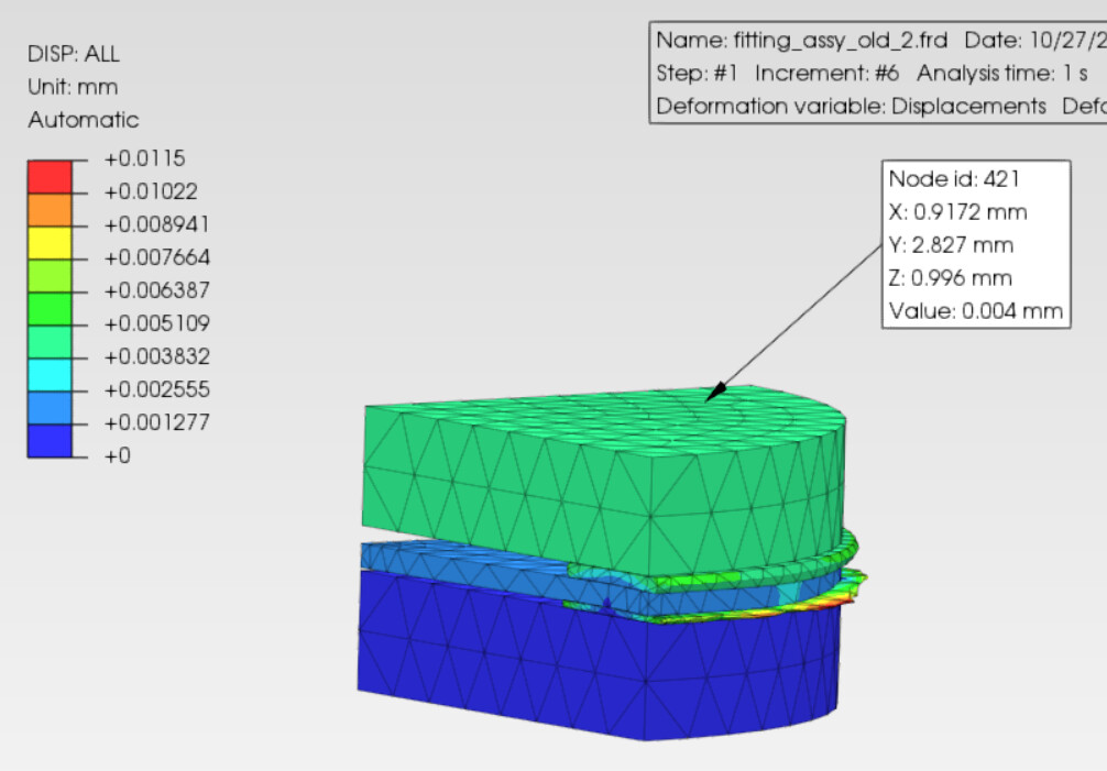
In this example, I apply a displacement of -0.004 mm in the Z direction. However the non linear result comes up with a displacement of 0.0115mm
Increment 1 has a displacement of 0.0006883
Increment 2 has a displacement of 0.001368 …getting close!
Increment 3 has a displacement of 0.002327 …half way there!
Increment 4 has a displacement of 0.003567 … almost there!
Increment 5 has a displacement of 0.007145 … Elvis has left the building!
Increment 6 has a displacement of 0.0115 … Thanks for all the extra data my friend!
Then you switch NLgeom off and set incrementation to Default and the result is exactly -0.004 at the surface that was displaced by -0.004mm I don’t understand what the difference is.
Your file has a prescribed displacement of U3=-0.001mm.
I’m new user and result window doesn’t go directly to the last step. It has puzzled me at the beginning. Maybe that’s the reason why you see a strange value. Be sure to query last increment of last step.
A displacement ALL is the magnitude of the displacement vector. If there is any displacement in the transversal direction, it adds to the displacement magnitude. That is why it is larger than the prescribed displacement, which was 0,001 mm in your shared file.
I am not sure to understand, what are axisymmetric elements? Are you recommending performing the analysis in a 3D Model Space? Do you specify anything about the thickness on the soft ? May I ask you how did you constrained your geometry - which BCs did you use ?
Also, you seem well informed so I may ask. If the symmetric slice of the model extends to the Y axis, should it require any further BC ?
I see the error in my ways. I wasn’t querying on the surface. I feel like the boy who cried wolf now, but I’m going to double check my other simulation results to see if I really did this or if something is really wrong.
so here is the tests from yesterday with large deformations on and 0.001mm and 0.004mm displacements showing the correct displacement.
I figured out why my previous attempt with more complexity didn’t reach the correct displacement. The solution says its complete, however, the increments never reached 1s. Instead the last increment says “solution contains NAN” values. So I take it, I need to do something. I’m currently playing around with the size of the initial increment. I had started with a very small initial increment 0.015s. I’ve increased that to 0.3s… and waiting to solve.
Ok, I’m back to square zero on this gasket analysis. So you are saying that I should do this as a standard “Model space: 3D, Unit system: mm, ton, s, °C”. Then what? import the model as a thin wedge? or as a thin, section? and to simulate the cylinder? only one part actually goes through the center axis, so how can the symmetry wall boundary conditions be simulated?