Comparing material stress-strain curve with uni-axial tension test analysis

[Cimek]

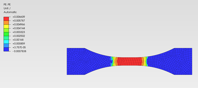
I’m testing the new Johnson-Cook material model so I made a square cube model meshed with 6 parabolic tetrahedron C3D10 elements. I applied symmetry constraints to 3 sides to prevent rigid body motion and displacement to one face.

I requested history output for Stresses, strains and plastic strain so that I can create stress-strain plots in excel. Now if I define my material as bi-linear elasto-plastic (no Johnson-Cook here) using the user interface (I enter the data points for the plastic stress strain curve) and I the also plot this curve in excel it matches perfectly with the curve I get from plotting the history outputs stress-plastic strain.

The problem is that if I try defining the material as Johnson-Cook (dynamic explicit step) and I try plotting it in excel using the equation below the plot does not match the one exported using history output.

I know that this model is strain rate and temperature dependent so I matched the temperature in excel and PPM and calculated the strain rate using the equations below, so it should also match. For the time and therefore velocity I varied the step time period and corrected the amplitude, so that the displacement ramps through the entire step duration. Am I wrong in how the strain rate is defined? Because if I change the time period and amplitude the history output stays the same. What am i doing wrong here?

test file:
Tensile_test_single_element_1.pmx (312.0 KB)

[FEAnalyst]

It might be better to ask on the CalculiX forum, there you may even get the reply from the developer of CalculiX (and you can create a GitHub issue in ccx repository if it seems to be a bug).

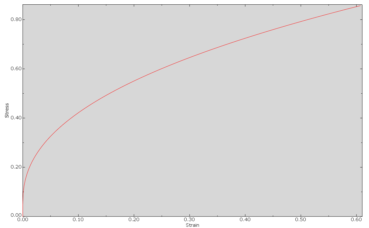
Here’s the curve that I obtained in Abaqus for the model in your file:

It would be better to use a single hex element. I know that it can’t be created in PrePoMax but you could import such a mesh. It could be even defined manually in the input file.

[Cimek]

Thanks I will copy this post to the CalucliX forum. Could you export the data points from your plot from Abaqus, so I could plot it on the same plot in excel? And how did you obtain it, did you replicate the same analysis?

[FEAnalyst]

@Cimek

Could you export the data points from your plot from Abaqus, so I could plot it on the same plot in excel?

Yeah, sure. Here they are (in strain (X) - stress (Y) format):

0	0
2.47943E-05	0.0497817
0.00066254	0.0933261
0.00241222	0.124444
0.00478155	0.150466
0.00750458	0.17187
0.0104805	0.190925
0.0136374	0.207809
0.0169272	0.223204
0.0203205	0.2373
0.0237623	0.250275
0.0273033	0.262544
0.0308933	0.274135
0.0344852	0.285028
0.0381453	0.295501
0.0417996	0.3054
0.0455163	0.314918
0.049214	0.323926
0.0529228	0.332592
0.056679	0.341026
0.0604021	0.349102
0.0641697	0.357009
0.0679365	0.364648
0.0716612	0.371977
0.0754193	0.37912
0.0792055	0.386104
0.0829451	0.392828
0.0867114	0.399423
0.0904689	0.40586
0.0942165	0.412132
0.0979524	0.418251
0.101714	0.42428
0.105423	0.430075
0.109156	0.435795
0.112875	0.441386
0.116581	0.446855
0.120309	0.452261
0.124023	0.457561
0.127684	0.462694
0.131365	0.467781
0.135068	0.472811
0.138718	0.477689
0.14239	0.482523
0.146044	0.487254
0.149683	0.491902
0.153304	0.496466
0.156945	0.500987
0.160534	0.505389
0.164142	0.509767
0.167733	0.514063
0.171342	0.518335
0.174899	0.522493
0.178474	0.526618
0.182032	0.530683
0.185573	0.534682
0.189098	0.538617
0.192606	0.5425
0.19613	0.546359
0.199638	0.550151
0.203129	0.553896
0.206603	0.557581
0.210093	0.56125
0.213566	0.56487
0.217022	0.568435
0.220462	0.571951
0.223885	0.57542
0.227291	0.578842
0.230713	0.582254
0.234119	0.58562
0.237507	0.588936
0.24088	0.592215
0.244267	0.595486
0.247638	0.598711
0.250962	0.601866
0.254331	0.605038
0.257654	0.608144
0.26096	0.611212
0.264281	0.614268
0.267586	0.617291
0.270876	0.620283
0.274149	0.623237
0.277437	0.626183
0.280679	0.629072
0.283936	0.631947
0.287176	0.634793
0.290431	0.637636
0.293641	0.640419
0.296865	0.6432
0.300045	0.645925
0.303239	0.648642
0.306446	0.651354
0.30961	0.654019
0.312787	0.656677
0.315921	0.659284
0.319069	0.661884
0.32223	0.664483
0.325348	0.667036
0.328452	0.669559
0.331569	0.672079
0.334671	0.674576
0.33776	0.677049
0.340861	0.679518
0.343921	0.681939
0.346994	0.684364
0.350052	0.686763
0.353097	0.689136
0.356128	0.69149
0.359145	0.693823
0.362175	0.696152
0.365191	0.69846
0.368194	0.700749
0.371183	0.703013
0.374159	0.70526
0.377147	0.707507
0.380121	0.709729
0.383057	0.711917
0.386031	0.714122
0.388966	0.716286
0.391888	0.718437
0.394823	0.720583
0.397744	0.722713
0.400653	0.724824
0.403549	0.726915
0.406432	0.728993
0.409327	0.731066
0.41221	0.733127
0.41508	0.735166
0.417937	0.737192
0.420783	0.739199
0.423616	0.74119
0.42646	0.743183
0.429293	0.745158
0.432113	0.747119
0.434922	0.749063
0.437718	0.750993
0.440526	0.752922
0.443322	0.754837
0.446106	0.756738
0.448879	0.758623
0.451639	0.760494
0.454389	0.76235
0.457149	0.764209
0.459898	0.766051
0.462636	0.767882
0.465362	0.769697
0.468077	0.7715
0.470803	0.773304
0.473496	0.775079
0.476199	0.776857
0.478892	0.778621
0.481573	0.780373
0.484266	0.782126
0.486925	0.783852
0.489596	0.785581
0.492256	0.787296
0.494905	0.788999
0.497543	0.790692
0.500192	0.792384
0.50281	0.794052
0.505438	0.795722
0.508055	0.79738
0.510662	0.799027
0.513259	0.800663
0.515866	0.802299
0.518442	0.803912
0.521029	0.805528
0.523605	0.807132
0.526171	0.808725
0.528728	0.810308
0.531294	0.811893
0.53383	0.813454
0.536377	0.815019
0.538914	0.816573
0.541441	0.818116
0.543978	0.819662
0.546486	0.821185
0.549003	0.822711
0.551512	0.824227
0.55401	0.825734
0.556499	0.82723
0.558978	0.828717
0.561468	0.830207
0.563929	0.831675
0.5664	0.833146
0.568861	0.834607
0.571313	0.83606
0.573775	0.837515
0.576209	0.83895
0.578653	0.840387
0.581087	0.841815
0.583512	0.843234
0.585929	0.844645
0.588336	0.846047
0.590753	0.847452
0.593142	0.848837
0.595541	0.850225
0.597932	0.851604
0.600314	0.852976
0.602705	0.85435
0.605071	0.855705
0.607429	0.857055

@Cimek

And how did you obtain it, did you replicate the same analysis?

I modified the syntax of this input file since Abaqus uses slightly different syntax and submitted the analysis there. So nothing was changed in model definition. Then I plotted average PEEQ vs average S22.

[Cimek]

I tried posting on the Calulix forum, but my question is pending for approval by a mod for 2 full days already. How long does this usually take?

And I tried plotting your Abaqus results and they don’t fit neither my results using Caluclix nor the theoretical curve plotted in excel using the Johnson-Cook equation with the same parameters. My guess is I’m somehow not calculating strain rate correctly. Do you have any experience calculating it?

[ANYS]

HI Cimek,

Regarding Plasticity with Johnson-Cook hardening Manual says:

" it has been implemented as a Abaqus Material User Subroutine in CalculiX, establishing a relationship between the corotational Cauchy stress and the corotational logarithmic strain"

That means strains shown on that formula are Logarithmic Strains in a similar way as they are input for the True Stress / True (Logarithmic) Strain curve for plasticity.

Your initial Strain Rate looks like it’s being derived from an Engineering Strain AL/L0. I’m not sure that’s correct ¿??. Appling the same criteria it should be defined as a Logarithmic strain rate ¿isn’t it?

Anyway, I would like to hear comments from the CalculiX forum as that formula is split into three depending on the strain rate evolution and

The term:

Is suspiciously similar to a Logarithmic Strain rate (Ln(Stretch Rate)).

Looks suspiciously similar to an Enginieering strain rate ( (Stretch Rate)-1).

Seems like the algorithm is splitted and mixes different strain formulations?¿?¿?

Regarding your plots it would be convenient you add the strain formulation you are representing to the Strain description. You might be comparing apples with pears.

[Cimek]

Sorry I did not translate the upper plot form slovenian. The x-axsis is true plastic strain and the y-axsis is true stress on both plots. The solid black curve labeled with 0,05/s_25°C-eksperimentalno are experimental results from a tensile test with 0,05 strain rate and 25°C. The results were first obtained as engineering stress / engineering strain and were converted to true stress / true plastic strain using the following exuations:

I did not preform the aforementioned tensile test, I only took the data from the following paper:
https://www.researchgate.net/publication/341604393_Effect_of_the_Temperature_and_Strain_Rate_on_the_Tension_Response_of_Uncured_Rubber_Experiments_and_Modeling

There is also data from other tests at different strain rates and temperatures in the paper that I also converted, I only posted one here, so that the lines are clearer.

It would be nice if PrePoMax/Calculix could output strain rate for a direct comparison.

Now that you mention that the formula is split into three i wonder if I would try plotting these three in excel if one of them would fit the Calculix results. But that would mean that the results are deviating from the default formulation or am I wrong?

[FEAnalyst]

This input file will be better for those tests (it’s a single C3D8R element):

*NODE, NSET=NALL
1,  0, 0, 10
2,  10, 0, 10
3,  10, 0, 0
4,  0, 0, 0
5,  0, 10, 10
6,  10, 10, 10
7,  10, 10, 0
8,  0, 10, 0
*ELEMENT, TYPE=C3D8R, ELSET=EALL
1,1,2,3,4,5,6,7,8
*SOLID SECTION, ELSET=EALL, MATERIAL=JC
*MATERIAL, NAME=JC
*ELASTIC
10, 0.47
*PLASTIC, HARDENING=JOHNSON COOK
0.05, 1, 0.43, 0.45, 130, 25
*RATE DEPENDENT, TYPE=JOHNSON COOK
0.087, 1
*DENSITY
1.52E-09
*NSET, NSET=Y_MINUS
1,2,3,4
*NSET, NSET=Y_PLUS
5,6,7,8
*NSET, NSET=X_MINUS
1,4,5,8
*NSET, NSET=Z_PLUS
1,2,5,6
*BOUNDARY
X_MINUS, 1, 1
Y_MINUS, 2, 2
Z_PLUS, 3, 3
*AMPLITUDE, NAME=AMPL
0, 0, 1, 1
*STEP, INC=100000
*DYNAMIC, EXPLICIT
2e-3 ,1, 2.8e-3
*BOUNDARY, AMPLITUDE=AMPL
Y_PLUS, 2, 2, 1
*EL FILE, FREQUENCY=1
S,E,PEEQ
*NODE FILE, FREQUENCY=1
U
*EL PRINT, ELSET=EALL, FREQUENCY=1
S,E,PEEQ
*END STEP

Of course, you can modify the strain rate or whatever else you want to check. You’ll just have to adjust the incrementation (and maybe output frequency) settings accordingly.

[ANYS]

¿Have you noticed your formula is different from the one in the manual?

The initial Strain rate is the total not the plastic.

[Cimek]

I did not, thanks for pointing this out. I checked the original paper from Gordon R. Johnson and William H. Cook “A constitutive model and data for metals subjected to large trains, high strain rates and high temperatures.” and it says the part in the logarithm is plastic strain rate, but the symbols in the equation are without the p subscript.

This would imply that my equation is correct. This begs the question what is actually used in ccx.

I think we might have just found the problem, I analytically calculated the total strain rate but it should be plastic, because plastic strain rate is probably used in calculix. So how do I analytically calculate the plastic strain rate?

[FEAnalyst]

Here’s the equation used by Abaqus:

[ANYS]

Hi,

I have also been doing some testing with the new Johnson-Cook model. It involves variables that I have not normally worked with (Strain Rates) and it has been difficult for me to understand how it works.
I have succeeded and also I think I have identified the mistake you might be doing because something similar has happened to me.

I am using a NLGEOM dynamic analysis in a tensile test on JohnsonCook_OFHC Copper at 10m/s which is equivalent to a true strain rate of 10.000 [s-1] in my model.
This value is similar to one of the three values suggested in Johnson Cook’s original paper for the OFHC COPPER.
My model is a 1mm1mm1mm cube. The result of the analysis coincides exactly with the theoretical curve of the model and the experimental values up to a PEEQ of 0.5. Beyond that my model starts to show necking, the values of peeq and VM vary locally and the comparison is no longer possible.
My result considers the isothermal process. I intend to test the adiabatic test using a Taylor-Quinney coefficient but later.

Here are the three main keys to solve the problem.

1-You should have very clear about the type of strains you are dealing with in order to correctly construct the theoretical curve and extract the ccx data.
The Johnson-Cook curves are for constant (I repeat: constant) True Strain Rate Equivalent value. They are using 1000, 10000 and 100000 [s-1].
That means you need to prepare your model in ccx and stretch it by imposing boundary conditions in such a way that the True Strain Rate remains constant the whole test.

-To avoid inducing waves that travel through your material, it is convenient to impose an initial velocity on the specimen such that it already has the necessary True Strain Rate from the first step.

*INITIAL CONDITIONS,TYPE=VELOCITY
TOP1,3,10. (m/s)

*INITIAL CONDITIONS,TYPE=VELOCITY
TOP2,3,7.5 (m/s)

*INITIAL CONDITIONS,TYPE=VELOCITY
TOP3,3,5. (m/s)

*INITIAL CONDITIONS,TYPE=VELOCITY
TOP4,3,2.5 (m/s)

-Adjust the total analysis time so that you do not exceed a PEEQ of 0.5 or the model starts necking. Track the Jacobian and check that it does not exceed above 1.01 or so.
The first test was with a very low True Strain Rate of 0.5 to understand my model and then I tightened it up up to 10000 [s-1].

This has worked for me:

*DYNAMIC,SOLVER=PARDISO
5E-08,5E-05,0,5E-08