Material Data for plastic / elastic model

I am digging into the field of non-linear static analysis.
As i’m not a specialist for material problems i need some advice from expierienced users regarding the use of plastic / elastic material model.

I’v read some posts, in this forum and on a blogs to the topic: How to derive plastic strain / stress data that can be used as Material model for FEM.
PreProMax Post
Blog Post

I have followed the procedure of both authors and have come to different conclusions.

When i compare the stress/strain curve from Datsko it seems, that it is still engineering stress/strain because the stress/strain data i derived from the Blog Post (H.N.Hill Equation) is true plastic strain vs true stress (see diagram above).

My questions are:

  1. Do i need to transform the stress/strain from the Datsko approach to true stress/plastic strain that i can use it in a plastic material model in ccx?
  2. Is the approach from the Blog Post (H.N. Hill Equation) + transformation to true plastic strain / true stress suitful for a plastic material model in ccx?

Thanks in advance
Eric

According to the cited forum post, yes. CalculiX needs true stress vs true plastic strain. Do the conversion and see if it fits the blog post data.

Why not. As long as you get reasonable true stress vs true plastic strain data, you can test it with CalculiX (possibly on a simple, maybe even single element model).

1 Like

Thank you for the fast answer.

I have calculated true plastic strain from the Datsko approach.
It is showing a quite different charakteristic compared to N.H.Hill equation.
Datsko approach seems to be more conservative than N.H.Hill approach.

Is it important to have a stess value for 0 plastic stress in the material definition in ccx, or is it exrapolating to 0 anyway?

Best Regards
Eric

Maybe you could find full experimental stress-strain curve for your material in literature. Those approximate approaches may indeed differ significantly.

The first plastic data point should be yield strength vs 0 plastic strain. Abaqus enforces that, CalculiX may not throw an error but it should still be done this way.

Thank you very much for clarification and recommendations!

Maybe I’m understanding incorrectly Mr. Datsko notes, or I read wrong your results, but I see some unexpected things.

According to Mr. Datsko notes there are some points that could be anticipated on the graph and can help to check if your curve is correct:

imagen

1-For a True plastic Strain of 1 (ew=1) —> Syw=Sigma0

Where ew=true plastic strain.

According to Datsko Sigma0=158033 Psi = 1090 MPa

Your last graph is showing you reach aprox 1100MPa>1090Mpa @ 0.09 True Plastic Strain. That’s seems too soon.

2-The instability point or maximum load condition is reached at , True plastic Strain 𝜀# = m

Su is an ultimate Tensile Strength (Engineering value) so you need the Engineering curve to check that against True Plastic Strain.

According to Datsko m=0.0371

3-Your Engineering curve (blue Datsko eng) doesn’t show instability point.

That’s a point in which the enginieering curve starts decreasing. A small amount of additional stress beyond that value results in infinite strain.

It helps a lot to plot clearly which Stress and Strain measure are you considering at every moment. Engineering or True. Plot up to ew=1 and both curves on the same graph.

I’m reading your blog Post and I can see:

Ultimate Tensile Strength is the point in which Global Strains become local in the tensile test (Necking begins). Point (3). It is an unstable Point. If your model is force driven, it will collapse.

Maximum elongation is associated to the Strain at the Fracture point (5)

I don’t understand why the blog Post is correlating those two values as if that were a point. Sound weird to me and it is expected both curves end up different. I’m not saying it’s wrong. Maybe it is a conservative hypothesis

Mr.Datsko imposes Instability point is a maximum (Derivative=0) to determine the curve we are searching for.
.

This is how Datsko aproach looks like to me.

Veeeery flat.

I would like to post some comments to clarify the approach to model plasticity.

The Stress - Strain relationship for strain hardening materials first proposed by Hollomon is : The most commonly used constitutive equation is the Hollomon equation, which has the form of a power-law relation between true stress σ and strain ε; σ = K ε^ n , where K is the strength coefficient and n is the strain-hardening exponent (Dieter, 1961, Hollomon, 1945, Kleemola and Nieminen, 1974). (Constitutive equations optimized for determining strengths of metallic alloys - ScienceDirect)
.
What my professor Datsko did was rename K to Sigma zero, and n to m. He then worked out the coefficients that need to be obtained from a tension test. His work described in my post allowed the calculation of the strain hardening exponent “n” from the relationships between the Yield Stress (Sy) and the Tensile Strength (Su). Datsko’s correlation Su/Sy = (184.m)^m

Datsko indicated that this relationship is valid for calculated values of m <=0.05.

The wrong interpretation occurs when it is not considered that the true stress-true strain behavior of a metal is the locust of the yield stress, that is, is a material is deformed to a true plastic strain Ew, when it was subjected to a true stress Sw, then its cross sectional area is reduced to Aw. Then if the stress is released and a new tensile stress performed, the initial cross sectional area for the new tensile stress is Aw, and if pulled in tension, its new Yield Stress will be Sw.

Therefore, in the equation Sw=K(Ew)^n represents the true stress-true strain work hardening equation of the material.

Calculix requires that the initial Yield stress will corresponds to a plastic deformation of 0.00, what I do is I assign the calculated Yield Stress at 0.002 to equal to the Initial point of the plasticity data, i.e., assign it the value 0.00. Since the true Yield stress for all the calculated values are used the implicit error is minimal.

That is not correct. You are missing the point:
The true fracture strain is Efracture = Ln (Cross sectional area initial/Cross Sectional Area at fracture). The deformation based on elongation is not valid when the Ultimate load is reached.
The true strain is always defined in a tension test as Ew= Ln (Ao/Ainst)
Constancy of volume results in Ao.Lo = Ainst.Linst or (Ao/Ainst)=(Linst/Lo)
However, after the maximum load is reached, the deformation concentrates in the neck formed and the deformation is not longer uniform

I was pretty sure that was going to open a beautiful debate although there is not too much people willing to talk about plasticity. :grinning_face:

Could I ask you two things?

1-What would be according to you the right curve known the given parameters so we can compare.?

E=200000 MPa (SORRY EDITED FROM 210000 to 200000)

Sy=856 MPa

Su=925 MPa

E0=0.002

2-Could you quote my wrong sentence. I’m not sure to understand if you refer to the Blog section or Mr. Datsko section.?

I never really had feed back on this to confirm and I would really apreciate to get some foundation on my procedure.

Tanks in advance and for joining again in this subject . You have been part of this from the beginning..

Here are the details
Procedure to calculate Strain Hardening exponent-rev.zip (660.4 KB)

Thanks FrdLorenzo ,

The procedure described in your link (Mr.Datsko proccedure) fits mine.

Regarding the procedure stated in the Blog Post : https://learnfea.com/stress-strain-curve-approximation-2/

What do you think about stating that maximum elongation is reached at UTS to determine the curve?


Regards

ANYS,
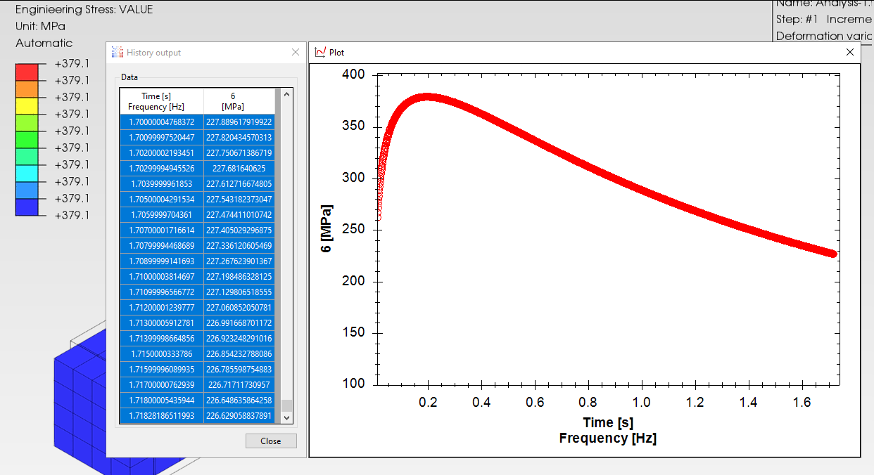
A tensile testing machine plots Load versus the machine’s crosshead extension. That is the plot that you have above. In a tension test an extensometer is added to determine the yield point, but is normally removed after that.
You can “convert” to engineering Stress vs. extension or even to nominal strain by converting the nominal strain = (Lo + Extension)/Lo where Lo is the original Gauge Length (normally 2 inches or 1 inch, or 50 mm or 25 mm)

The %Elongation which is not a material property since it depends on the gauge length used in the test. The measured %Elongation for a 25 mm gauge length will by larger than for a 50 mm gauge length because it will reflect more the effect of the “necking” that develops after the Ultimate load is reached.

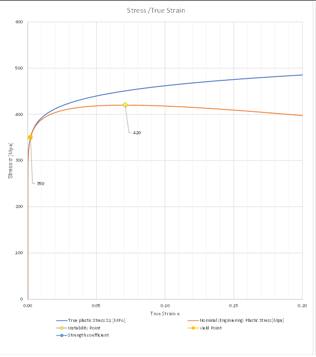
If the True stress (Li/Ai) where Li is the instantaneous load and Ai is the area corresponding to Li is plotted vs. the true strain defined as Ei = Ln(Ao/Ai) where Ao is the original cross sectional area, there will be no instability since the true stress will continue to increase as the cross sectional area decreases rapidly after the instability or maximum load is reached.

The instability that develops during a tensile test is well documented in the scientific literature, and when the Hollomon or Datsko Strain hardening equation is used to define the relationship between True Stress and True Deformation is used, the result is that the plastic deformation at instability, that is at the maximum load in a tension test equals m, the strain hardening exponent.

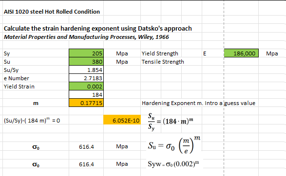
Datsko’s work clearly shows that if the Yield Strength and the Tensile Strength are known from a simple tension test, the the strain hardening exponent can be easily determined using my Excel suggestion or by trial and error using using the equations indicated.

I strongly disagree when the Blog states that determining m - the strain hardening exponent is difficult.

Furthermore, using the maximum elongation and matching it to the instability or point of maximum load simply shows poor understanding of mechanical properties of metals. I reiterate that the % reduction in area or %AR is the true measure of the ductility of the material. The fracture strain, which is used in metal forming plasticity Efracture = Ln (100/100-%AR) is the value that matters.

In Datsko’s book listed in my references Datsko writes that you can define the total strain as
Et = Ee +Ep (total strain equals Elastic def. plus Plastic Def)

Now if the deformation is only elastic, then
Ee = Stress/Young’s modulus = Sigma/E

And in the plastic portion

Et= Ee +Ep = (Sigma/Sigma_zero)^(1/m)

or Ep = (Sigma/Sigma_zero)^(1/m) - Sigma/E

this is the Ramberg–Osgood relationship and shows that the strain hardening exponent in the Ramberg–Osgood is simply the inverse of Datsko’s strain hardening exponent.

In his book, (I am trying to attach the plot in Log-Log coordinates) Datsko shows strain hardening curves for elastic plus plastic deformation and just the plastic deformation. The expected result is that when the plastic deformation is large the value of the elastic deformation does not affect the result of the calculation.

He points out that if the total strain is used for 1020 Steel ( I do not know where you are, but this is Carbon steel with .2% carbon) the curve fit is 120000 (Et)^0.22 and if Ep is used the equation is 121000 (Ep)^0.21. The numbers obtained for Et=0.002 and Ep=0.002 are approximately 30000 psi and 32000 psi. Obviously, for larger plastic deformation the values will be very similar if not identical.

ANYS, I sincerely hope that this comments have cleared some of your questions but feel free to contact me if you have more questions or ideas.

Best regards
Datsko’s-plot.zip (510.6 KB)

Et= Ee

Thank you very much FdoLorenzo for your detailed and comprehensive response.
I will look into detail each paragraph to compare with my expected curve and actual understanding.

¿Could you please help me to find the right material source?
I’m not used to that designation and a quick search doesn’t agree with the data. I’m doing kind of reverse enginiery to derive Sy and Su from m and so. I think it’s important to agree on the starting material parameter to see if we both end up in the same curve.

According to the graph and depending the value of m finally used the material parameters are:

Thanks in advance

1 Like

ANYS,

The data that you found for AISI 1020 is not in the annealed or hot rolled (softer) condition. That 1020 steel is either heat treated or cold worked (Deformed) to have those values.

That material has the curve shown in the appended plot, and an m value of 0.0708.

The vlaues that you plotted that you took from Datsko’s plot are for annealed 1020 steel, and if you recall Datsko indicated that the equation predicting the Yield strength of 32539 was using the plastic strain, and the one predicting Yield Strength of 30578 was using the total strain.

Although Sigma_zero and m allow the calculation/prediction of Sy and Su, the material condition which is described by Sy and Su only applies to that material.

That material taken from AZOM.com is not in the annealed or hot rolled condition.

Best regards,

FdoLorenzo

1 Like

ANYS Plot.zip (550.3 KB)

Hi and thanks again,

1-AISI 1020. (350 Mpa,420 Mpa)-- (0.0709,544)
We are in the same page in this case and for the area beyond 0.002 (Yield point).Note the small m value.


If I understand correctly minor differences come from if one considers 0.002 as total or as plastic strain.

2-Those large m values are still puzzling me.
AISI1020 annealed condition I still don’t understand how a material can reach up to a 22% of true plastic strain (m=0.22 according Datsko) at Ultimate Tensile Strength.


*Reprinted from Material Properties and Manufacturing Process by Joseph
Datsko. New York: John Wiley & Sons, Inc. , p 21.
https://www.osti.gov/servlets/purl/4703707

My numbers are;

a) m=.1 For AISI 1020 Steel, annealed at 870°C (1600°F), furnace cooled 17°C (31°F) per hour to 700°C, air cooled, 25 mm (1 in.) round Condition

b) m=.17715 For AISI 1020 Steel, hot rolled, 19-32 mm (0.75-1.25 in) round Condition


which is still far from the reported value.

1 Like

ANYS,

All the calculated values that you have are correct! 100% correct. Measured values are very specific to the sample that was tested.

The calculation of Sigma_zero and m allows you to model the plastic behavior of the case that you are modelling. Only materials in a specified chemical composition, condition of thermal treatment and grain size will yield similar results.
Consider for example that AISI 1020 steel can have the following composition range:
The chemical composition of AISI 1020 steel is;

|Carbon, C|0.17 - 0.230 %|
|Iron, Fe|99.08 - 99.53 %|
|Manganese, Mn|0.30 - 0.60 %|
|Phosphorous, P|≤ 0.040 %|
|Sulfur, S|≤ 0.050 %|

The carbon content will change the amount of the Ferrite and Pearlite phases and will change the yield and tensile strength of the sample. However, if the chemical composition is within the specified values, it classifies as a 1020 steel.
Young’s Modulus on the other side is constant or almost constant for all carbon steels and most aluminum alloys due to Iron and Aluminum comprising the highest component.
What I am trying to say is that the mechanical properties of all those steel samples are valid.
Now if you look at the table that you have in this post, Datsko’s 1020 steel had a measured value of 0.22. If you look to the right, it had a fracture strain of 0.9.
What this means is that if your sample had an initial diameter of 10 mm, you can pull it in tension to a diameter of 8.95 mm to reach m (plastic deformation at maximum load) but at the failure point in the tension test the sample’s diameter would have reduced to 4.07 mm.
I hope this help!
By the way, I am in Spring, Texas. Where are you located?

1 Like

Thanks again for accompanying the progress.

West Europe. Best city in the world close to mediterranean sea. :wink:

I’m going one step further.
I’m Using the AISI 1020 Steel, hot rolled, 19-32 mm (0.75-1.25 in) round Condition.
Once the Datsko parameters are clear I’m deriving the corresponding Rameberg_Osgood parameters to input into ccx *DEFORMATION PLASTICITY (Units in Pa, m).

*MATERIAL,NAME=Ramberg
**Young’s modulus (E).
**Poisson’s ratio (ν).
**Yield stress (σ0)
**Exponent (n).
**Yield offset (α).
**No temperature dependence is introduced
*DEFORMATION PLASTICITY
186000000000,.29,205000000,5.64495,1.81463

Everything is in good agreement with Datsko curve. Too good agreement in fact .
I say that because I would expect some necking initiation (deviation from the perfect behavior) beyond Ultimate Strength or Instability Point.

My model is displacement driven and there is no signal of necking. Apart from that all values are as predicted by the Datsko adjustment.

(*) I have scale the pure tensile test pseudotime to represent the Enginieering (Biot) strain (1.718 s). Last Point then becomes Logarithmic (Hencky,True) strain =1 .
Picture captures the closest instant in which PE=m=0.1774 . Expected Enginieering Stress value is ultimate Strenght value=380MPa

NOTE: By the way, I think Yield offset name for (α) is a very unfortunate designation because it may lead to confusion with the 0.002 Yield Stress offset. Also, because it is not an offset but a scaling parameter.